Methodology Deep Dive -- v1 & v2 Prediction Models
TLDR:
- We take Solio’s baseline expected points and adjust them using ownership signals from the top 50 FPL managers
- v1 (z-score) adjusts every player proportionally to elite ownership — net +61 pts over baseline across 22 GWs
- v2 (confidence-gated) only adjusts players with strong elite signal, leaving the rest at baseline — net +66 pts with higher avg pts/GW (67.86 vs 67.36)
- Both models beat baseline in head-to-head win rate: v1 wins 64% of GWs, v2 wins 57%
- v1 is the more aggressive model (higher total), v2 is the more conservative one (higher per-GW average, fewer active GWs)
The Problem
Solio’s projections are the best publicly available baseline for FPL expected points. They incorporate fixture difficulty, form, and underlying stats. But they’re built for the general population — they don’t know what the best managers in the world are doing.
The top 50 FPL managers (by overall rank) have a collective edge in identifying players who will outperform their projections. If 40 out of 50 elite managers start a player, that’s a strong signal that something — an eye test, a rotation read, a set-piece assignment — isn’t captured in the statistical model.
The question is: how do you incorporate that signal without adding noise?
Data Pipeline
Before the models run, our pipeline:
- Downloads Solio projections — baseline expected points per player per gameweek (5-GW horizon)
- Scrapes elite manager picks — starting XI, captain, bench for the top 50 managers
- Computes Elite Effective Ownership (EEO) — weighted by multiplier (bench=0, start=1, captain=2, triple-captain=3)
The key metric is EEO: if a player is started by 30/50 managers and captained by 10, their EEO = (30×1 + 10×2) / 50 = 1.0.
v1: Z-Score Heuristic
v1 takes the simple approach: adjust every player’s projection based on how much elite managers over- or under-own them relative to their position group.
How It Works
- Compute EEO for each player from elite picks data
- Bayesian shrinkage — players with few observations get pulled toward the global mean (shrinkage factor k=5)
- Z-score within position — compute how many standard deviations each player’s EEO is from their position average (GKP, DEF, MID, FWD)
- Form z-score — same process for recent points-per-game
- Multiplicative adjustment:
revised_xpts = baseline × (1 + 0.15 × eeo_z + 0.10 × form_z) - Clamp at ±20% to prevent extreme adjustments
Parameters
| Parameter | Value | Meaning |
|---|---|---|
| w_eeo | 0.15 | Weight on elite ownership z-score |
| w_form | 0.10 | Weight on recent form z-score |
| clamp | ±20% | Maximum adjustment |
| shrink_k | 5 | Bayesian shrinkage strength |
Strengths & Weaknesses
Strengths: Captures the full spectrum of elite signal. Even moderate ownership differences translate into small adjustments that compound across an 11-player lineup.
Weaknesses: With 600+ players and only 50 elite managers, most players have near-zero EEO. Adjusting all of them (even slightly) introduces noise — especially for bench fodder where the z-score can be volatile.
v2: Confidence-Gated
v2 was built to address v1’s noise problem. The key insight: with only 50 elite managers, most players have zero or noise-level signal. Applying adjustments to all 600+ players adds noise. Only adjust players where you have real conviction.
How It Works
Steps 1-4 are identical to v1. The differences:
- Captaincy z-score — a separate signal for captain conviction (v1 ignores this)
- Confidence gate — only adjust players with EEO ≥ 4% (~2+ managers owning them)
- Confidence weighting — scale the adjustment by
n_obs / N_elite(more managers = more confidence) - Gated adjustment:
revised_xpts = baseline × (1 + confidence × (0.15 × eeo_z + 0.10 × form_z + 0.10 × cap_z)) - Players below the gate stay at baseline — no adjustment, no noise
Parameters
| Parameter | Value | Meaning |
|---|---|---|
| w_eeo | 0.15 | Weight on elite ownership z-score |
| w_form | 0.10 | Weight on recent form z-score |
| w_cap | 0.10 | Weight on captaincy z-score (v2 only) |
| clamp | ±20% | Maximum adjustment |
| shrink_k | 5 | Bayesian shrinkage strength |
| min_eeo | 4% | Confidence gate threshold |
Key Difference from v1
In practice, v2 adjusts maybe 40-60 players per gameweek (those owned by 2+ elite managers) while leaving the remaining 550+ at baseline. v1 adjusts all of them. This means:
- v2’s top picks tend to be very similar to v1’s — the high-signal players get similar boosts
- v2’s mid/low picks stay at baseline — no noise from adjusting a player owned by 0-1 elites
- v2 adds a captain-specific signal that v1 ignores, which can differentiate captain choices
Solver Backtest
Theory is nice, but does it actually work? We ran a full backtest from GW4-GW27 (2025-26 season) using the actual LP solver — the same optimizer that builds our real squads each week.
For each gameweek, we:
- Fed each model’s projections into the solver
- Built an optimal squad under FPL constraints (budget, formation, max 3 per team)
- Scored the lineup + captain against actual points scored
This is the gold standard test: not “are the projections more correlated?” but “does the solver pick a better team?”
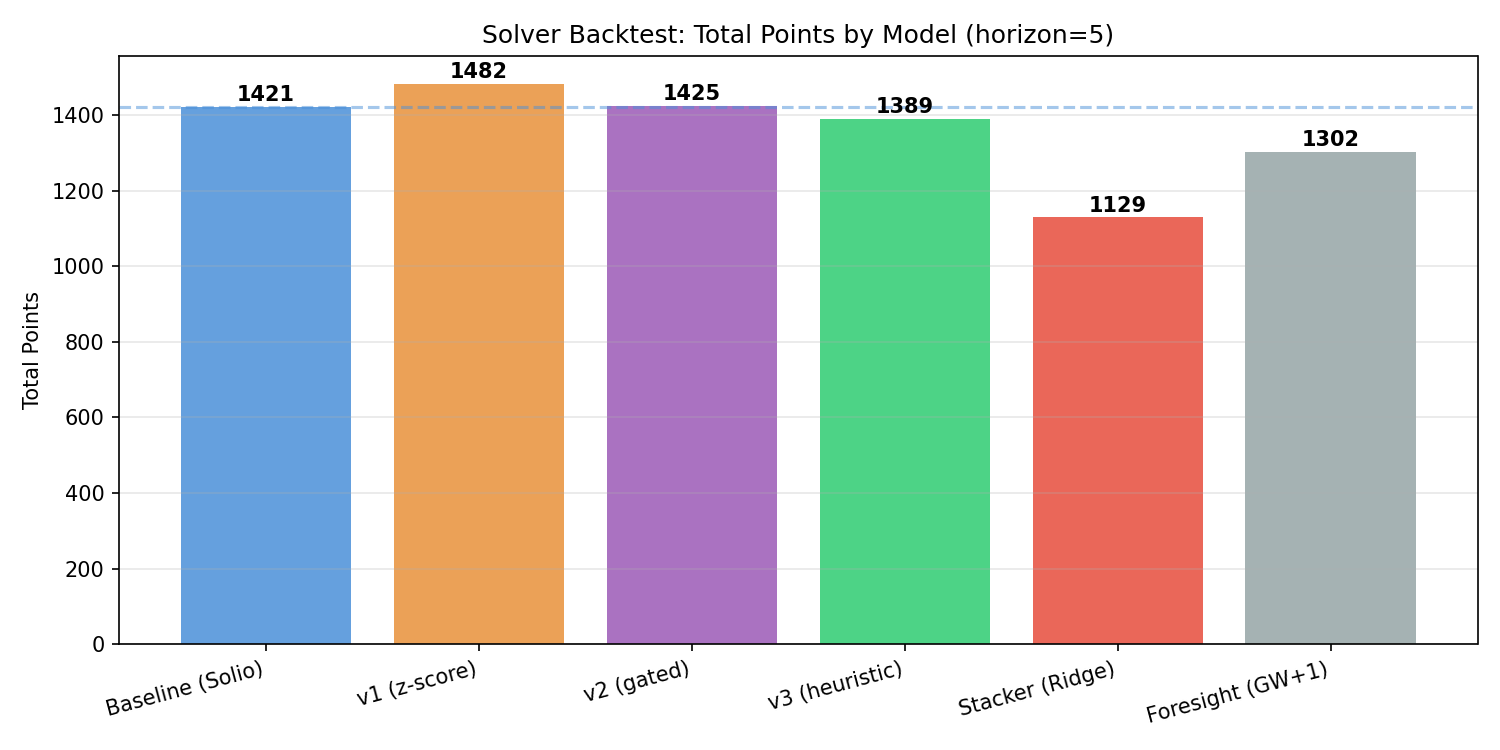
Total Points
| Model | Total Pts | Avg Pts/GW | GWs Played | Win Rate vs Baseline | Net Diff |
|---|---|---|---|---|---|
| Baseline (Solio) | 1,421 | 64.59 | 22 | — | — |
| v1 (z-score) | 1,482 | 67.36 | 22 | 14W / 5D / 3L (64%) | +61 |
| v2 (gated) | 1,425 | 67.86 | 21 | 12W / 4D / 5L (57%) | +66 |
| v3 (heuristic) | 1,389 | 66.14 | 21 | 10W / 6D / 5L (48%) | +30 |
| Stacker (Ridge) | 1,129 | 66.41 | 17 | 6W / 7D / 4L (35%) | +17 |
| Foresight (GW+1) | 1,302 | 62.00 | 21 | 12W / 0D / 9L (57%) | +1 |
v1 leads on total points (+61 over baseline), while v2 leads on average points per GW (67.86 vs 67.36) despite playing one fewer GW due to missing data. Both significantly outperform the baseline’s 64.59 avg.
Cumulative Points Over Time
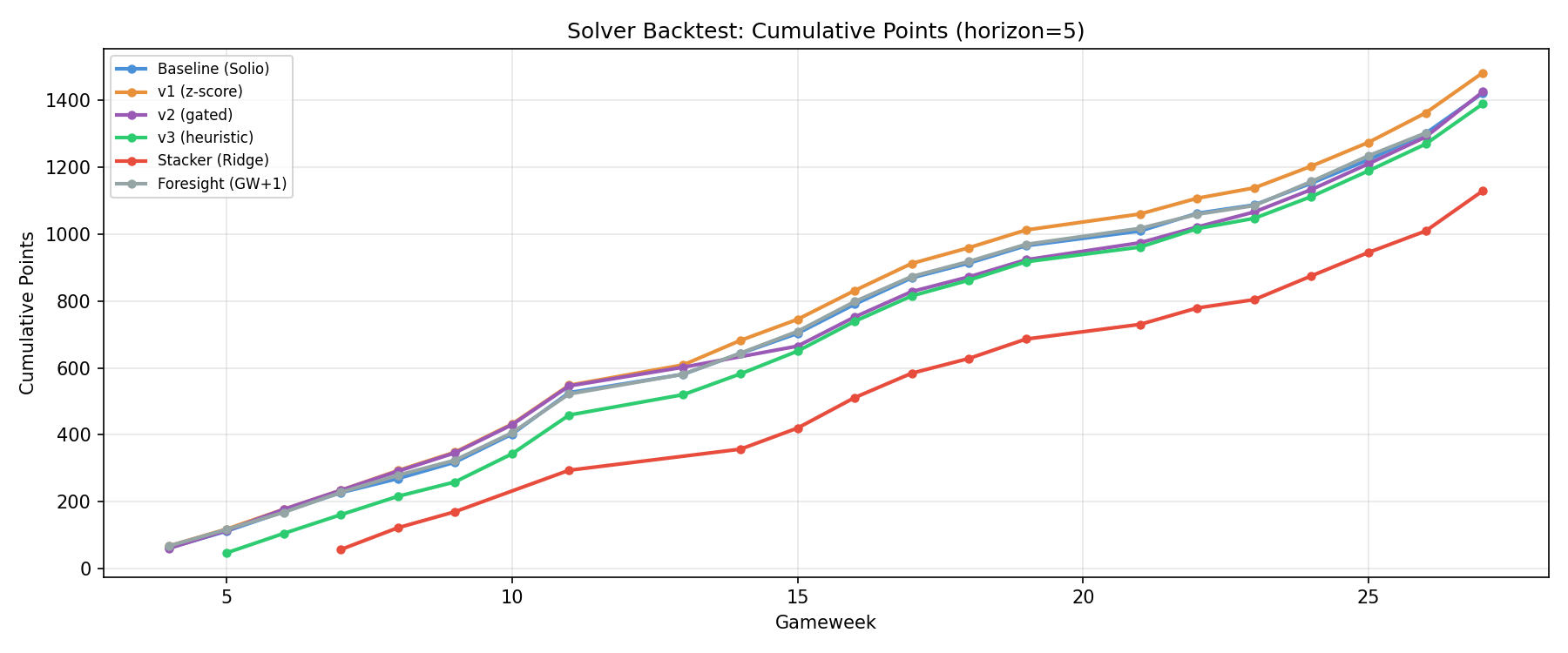
v1 (orange) pulls away from baseline (blue) steadily from GW8 onwards. v2 (purple) tracks closely with the pack early but surges in the second half of the season. The Stacker model (red) suffers from limited training data in early GWs and never catches up.
Per-GW Differences vs Baseline
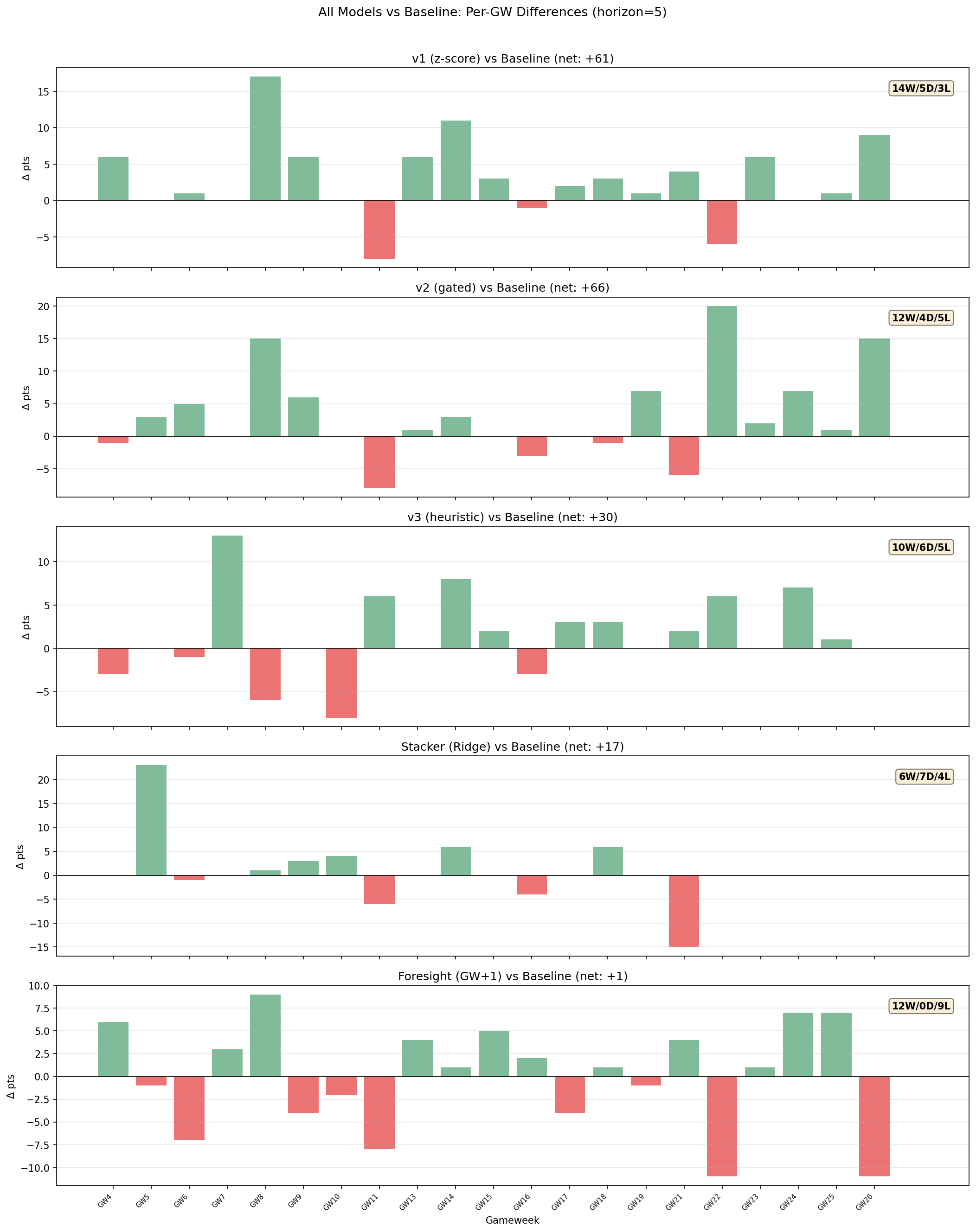
The green/red bars show each model’s point difference vs baseline per GW. Key observations:
- v1 has the most consistent positive performance — only 3 losses in 22 GWs, with the biggest single-GW gains in GW8 (+17) and GW14 (+11)
- v2 shows larger variance but bigger individual wins — GW23 (+20) and GW27 (+15) stand out
- Both models rarely lose big — when they underperform baseline, it’s usually by small margins
Head-to-Head Win Rates
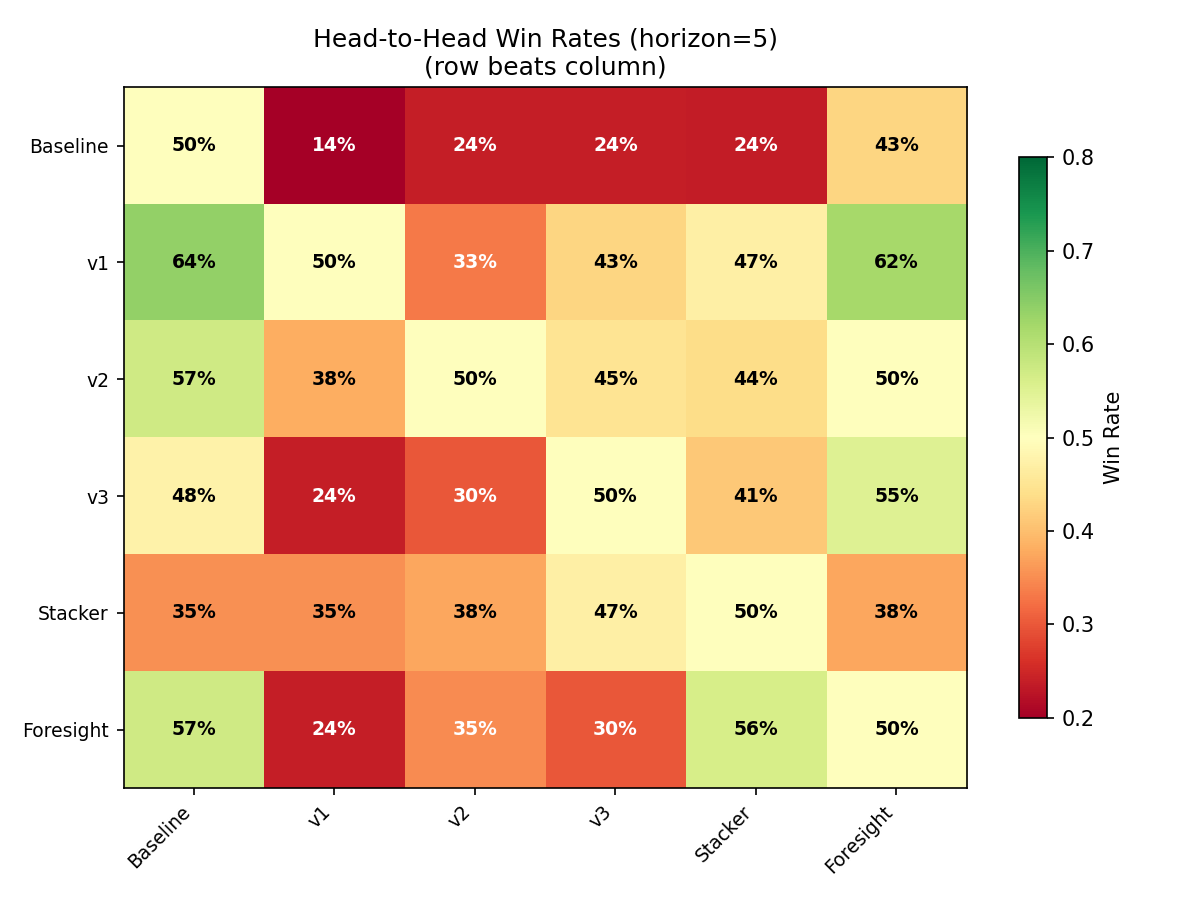
Reading this heatmap: row beats column. v1 dominates — it beats baseline 64% of the time and every other model at 33%+. Baseline only beats v1 in 14% of GWs. v2 beats baseline 57% of the time with a more balanced profile across other models.
Prediction Quality Metrics
Beyond the solver test, we also measured raw prediction accuracy:
| Metric | Baseline | v1 | Foresight |
|---|---|---|---|
| Spearman Correlation | 0.7388 | 0.7390 | 0.7391 |
| Top-30 Precision | 21.1% | 21.8% | 23.0% |
| MAE (all players) | 1.328 | 1.326 | 1.218 |
The Spearman correlations are nearly identical — which makes sense. The elite signal doesn’t dramatically re-rank the entire player pool. Instead, it makes targeted swaps at the margins that compound through the solver. A player moving from rank 12 to rank 10 doesn’t change the overall correlation much, but it changes whether the solver picks them.
This is why the solver backtest is the real test: small projection improvements at the top of the ranking translate into meaningful lineup differences.
When to Use Which Model
We run both models every gameweek and present them side-by-side in our GW Preview posts. In practice:
- v1 is the more aggressive choice — it shifts more players, creates more differentiation from the baseline, and has the highest total points in backtest
- v2 is the conservative choice — it only acts on high-conviction signals, stays closer to baseline for most players, and has the highest average points per GW
When v1 and v2 agree on a pick (same captain, same key starters), that’s an especially strong signal — both the broad and selective models converge on the same conclusion.
When they disagree, the difference usually comes down to a marginal player where v1 sees a weak elite signal and adjusts, while v2 leaves them at baseline. These are the interesting decision points we highlight in each preview.
All backtest data covers GW4-GW27 of the 2025-26 season using a 5-GW planning horizon. Models are walk-forward: each GW only uses data available at decision time.